OneModel syntax
The OneModel syntax simplifies the definition of SBML models and extends the functionality of SBML by introducing high-level elements. The models can be defined using base SBML elements such as parameters, species, reactions, rules (substitution, differential or algebraic equations); or using OneModel high-level elements such as functions, classes, inheritance. High-level elements, which do not have an SBML representation, are converted into equivalent low-level representations when the model is exported to SBML.
The following figure shows the typical structure of a model developed with OneModel. There are three main sections: import dependencies from previously defined models (line 1), the model definition (lines 2–8), and the standalone example (lines 9–11).
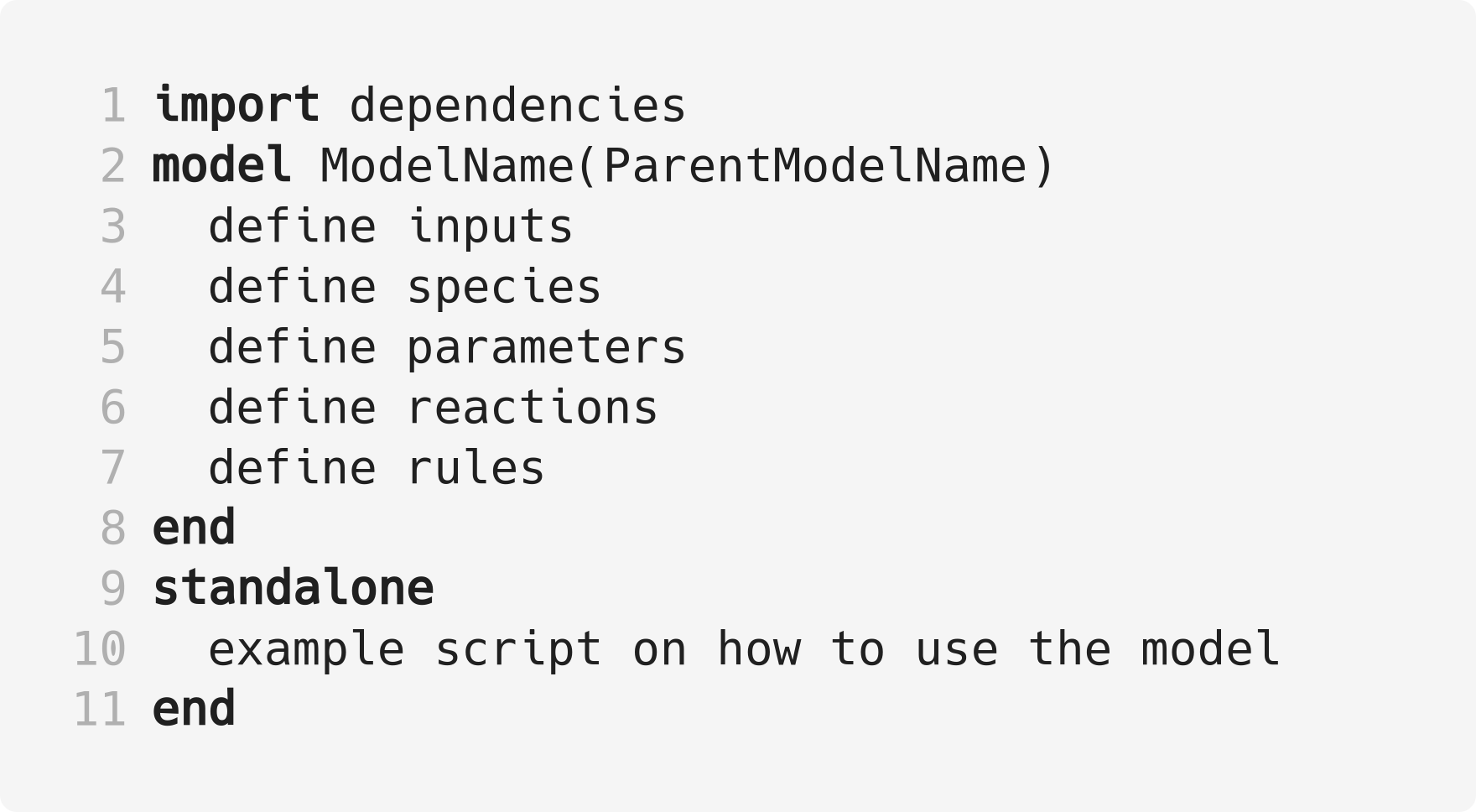
Fig. 7 Pseudo-code representing the structure of a model written with OneModel syntax. In line 1, the user can import previously defined models. In lines 2–8, the user can define one o more models using: inputs, species, parameters, reactions, and rules. The models might be an extension code of the ones previously defined. Finally, in lines 9–11, the user can define an example-of-use instance for the models in this file and within the standalone block.
The first section imports all the dependencies. Here, the user imports previously defined models to use and combine them as building blocks for developing more complex models or to extend their functionality.
The second section is the model definition.
In this section, several models can be defined using: (i) inputs, (ii) species, which can be interpreted both as chemical species and state variables, (iii) parameters used by reactions and rules, (iv) biochemical reversible and irreversible reactions, and (v) rules which can be substitution, differential or algebraic equations.
Models can extend the functionality of previous ones; for example the model with name ModelName will inherit all the elements (inputs, species, parameters, etc) of the parent model with name ParentModelName (line 2).
The last section is the standalone instance. Within this block, the user can define an example code that shows how to use the model (or models) defined above. It is important to note that the code inside the standalone block is not imported: the standalone code is only read when we export this model file directly. The advantages are: (i) each model file can always be exported as a standalone model allowing us to test each model individually for coherence, and (ii) the user always has an example of how to use the model.
We will briefly show the model-elements available in OneModel syntax in the following subsections.
Parameters
Parameters are time-invariant values that do not change during the simulation of the model.
They are used in the definition of the reaction rate constant and rules.
Parameters are declared using the keyword parameter.
The following code shows the different alternatives for declaring parameters.
# Parameters can be defined with a single-line command.
# Here we declare a new parameter 'k1' with value 1.
parameter k1 = 1

# We can also declare multiple parameters using commas.
# (if we don't set the value, the parameter is set to 0)
parameter k2 = -1, k3 = 3.14, k4 = 1e+5, k5

# Other alternative is to use a 'parameter' 'end' block, without using commas.
# This way be can comment easily the each parameter.
parameter
  # Transcription rate of mRNA. molec/min
  k = 1
  # Degradation rate of mRNA. 1/min
  d = 0.12
end
Note: parameters are saved in SBML as “parameter” elements.
Species
Species represent both (pseudo-)chemical and (pseudo-)biological species and state variables; values that change during simulation time due to reactions or rules.
Species are declared using the keyword species.
# Similar to parameters, species can be defined with a single-line command.
# Here, we declare a species S1 with initial value set to 1.
species S1 = 1

# We can also declare multiple species using commas.
# If we don't set the initial value, it will be set to 0 by default.
species S2 = -1, S3 = 1e-1, S4

# species also allows multiple declaration with a 'species' 'end' block.
species
  mRNA = 0     # mRNA concentration. nM/cell
  protein = 0  # protein concentration. nM/cell
end
Note: species are saved in SBML as “species” elements.
Reactions
Reactions represent a process in which the reactants are consumed to generate the products at a given reaction rate.
They are one of the ways to define how the value of the species will be modified during simulation time—being the other way to use rules.
If a species is present in a reaction (as a reactant or a product), the species value cannot be set by a rule and vice versa. The value of a species can only be set by (i) a set of reactions or (ii) one unique rule. If we define the rate of change of a species with a reaction, we cannot add a new rule which sets its value, but we can still add more reactions that interact with that species (as a reactant or a product).
Reactions are declared using the keyword reaction and are defined using the following syntax:
name: reactants -> products; rate
where name: is the name of the reaction (this is an optional part), reactants are the name of the species which the reactions will consume, -> is the arrow of the reaction and indicates the directionality of it, products are the name of the species produced by the reaction, ; is used to separate the reaction rate from the rest of the reaction, and rate is an equation (composed by parameters or species) which calculates the reaction rate.
If multiple species are consumed or produced at the same time, their names must be separated by a + sign.
# Reactions are declared within a 'reaction' 'end' block.
reaction
  # Species S is consumed to form P at rate k*S.
  S -> P ; k*S

  # mRNA transcription at a constant rate k_mRNA.
  0 -> mRNA ; k_mRNA

  # mRNA degradation proportional to mRNA concentration.
  mRNA -> 0 ; d_mRNA*mRNA

  # Antithetic sequestration.
  sigma + anti_sigma -> 0 ; gamma*sigma*anti_sigma

  # We can name a reaction writing its name followed by a ':'.
  # In this way we can refer to this reaction later in the code.
  R1: 0 -> A; k_A
end
Note: reactions are saved in SBML as “reaction” elements.
Substitution, rate, and algebraic rules
Rules represent three types of equations (substitution, rate, and algebraic equations), and they are used to define how the value of a species varies in simulation time.
They are declared using the keyword rule.
Substitution rules
Substitution rules are defined as name := equation and they are used to assign the value of a species with a mathematical expression.
The substitution rules are evaluated in each simulation step; therefore, the value of a species set by a substitution rule can change over time.
Note that substitution rules do not introduce new constraints in a model; they are just an assignment of the value of a variable.
For example, x_total := x_active + x_inactive is a valid substitution rule.
Algebraic rules
Algebraic rules are declared as name == equation and they are used to introduce algebraic constraints (the value of one species must hold a mathematical constraint during simulation time). The algebraic rules are evaluated in each one of the simulation steps.
In SBML algebraic rules take the form of 0 == equation, however in OneModel is necessary to explicitly write name == equation where name is the name of the species which the solver has to iterate to satisfy the algebraic rule.
For example, 0 == x_active + x_inactive - x_total is not a valid algebraic rule—we have to explicitly tell to OneModel which one of the species will have its value set by the algebraic rule—. Then, x_total == x_active + x_inactive is the valid form of a algebraic rule.
Substitution vs. algebraic rules
Substitution rules are mathematically equivalent to algebraic rules. However, the main difference is that the substitution rules are exact, and the value of the algebraic rules is solved numerically, so the accuracy of the result will depend on the error tolerances of the simulator.
Useful tips for working with algebraic rules…
If you can find an analytical solution for your model, use substitution rules instead of algebraic rules.
Algebraic rules are more challenging to simulate, and many simulators do not support them. Use algebraic rules as a last resort.
When using the quasi-steady state approximation, it may be difficult—or even impossible—to obtain an analytical solution of the derivatives of your model. In this case, it is unavoidable to use algebraic rules to set the derivatives to zero.
Rate rules
Rate rules are declared as der(name) := equation, and they are used to define the rate of change of a species over time (to set its derivative).
The following code shows an example of the use of each type of rule in OneModel.
# Rules are declared within a 'rule' 'end' block.
rule
  # Substitution rule.
  S := 10*s
  # Algebraic rule.
  # (note that this could be changed into a substitution rule).
  y == 10 - x
  # Rate rule.
  der(x) := S - x
  # As reactions, we can give a name to the equation with ':'.
  E1: z := x + y
end
Note: the rules are saved in SBML as “assignment rules”, “rate rules” and “algebraic rules” respectively. The value of a species can be set by a set of reactions or by a rule. It is not possible to combine both methods.
Model and objects
OneModel syntax implements modularity through class-based programming.
A class groups a set of model-elements (parameter, species, rules, etc.) under a class name.
Classes cannot be used directly to simulate; they are used to instantiate objects that will have a copy of each of the model-elements of the class.
A class is defined using the keywords model and end
An object is defined using the name of the class we want to instantiate, followed by ()
Classes can inherit the model-elements of previous classes. Inheritance is done by writing the parent class name in parentheses in the definition of a new class.
The following code shows an example of using classes and objects.
# Define 'Protein' model.
model Protein  # Start model definition.

  species protein

  parameter k = 1, d = 1
  reaction
    0 -> protein ; k
    protein -> 0 ; d*protein
  end

end  # End model definition.

# Define 'ProteinInduced'
model ProteinInduced

  # Extend the code of Protein into this model
  extends Protein

  species TF

  parameter h = 1

  rule k := TF/(h + TF)  # Override the value of 'k' with a rule.
end

standalone
  A = Protein()           # Instantiate an object of 'Protein'.
  B = ProteinInduced()    # Instantiate an object of 'ProteinInduced'.
  rule B.TF := A.protein  # Object properties can be accessed with '.'.
end
Note: classes are not saved in SBML, and objects are saved in SBML by saving their model-elements with a prefix related to the object’s name.
For example: the species A.protein will be saved as a species with name A__protein.
Import
OneModel syntax allows us to import code from other files into the current one using the keywords from and import.
The code from the imported file is executed as it were present in the current file, but the code inside the standalone block is omitted.
# To import a model, we have to write the path of the file we want to import
# relative to the current file path.
from 03_protein_constitutive import ProteinConstitutive

# The code inside '03_protein_constitutive.one' will be now accesible,
# and we can use the models defined in it.
A = ProteinConstitutive()
Note: SBML models do not support importation. When we export into SBML, all the model-elements from the imported files will be saved in the generated SBML.
Standalone
The code inside the standalone block will not be imported to other files: the standalone code is only executed when we run the model directly.
The standalone is declared using the keyword standalone and end.
# Here we define a model which we will import later into other file.
model MyModel
  species u
  species x=0
  rule x '= u - x
end

# In the standalone we can define an example to show how to use it.
# Another benefit is that all our models will run as a standalone model,
# making it easier to debug models and maintain them.
standalone
  myModel = MyModel()
  rule myModel.u := 10
end
Note: only if the model is directly exported into SBML (instead of importing it into another model), the contents of its standalone section are saved into the SBML.
Comments
Single-line comments start with a numeric hash symbol
#and finish at the end of the line. The following code shows an example OneModel code with comments.# SimpleReaction models a simple reaction. model SimpleReaction # Start definition of SimpleReaction. species A = 0, B = 0 # Define species A and B. parameter k = 1 # Define k as a parameter. reaction # Start reaction block. A -> B ; k*A # Conversion reaction. end # End reaction block. end # End the definition of SimpleReaction.Note: comments are not saved into the SBML files when the model is exported.